Polynomial equatios and solving them

Now that we’ve got a handle on some basic functions and their properties, we’re going to move on to
solving equations involving these functions. Such skills are useful in almost every conceivable application.
We’ll begin by considering a few different types of polynomial equations, and for each type of equation
we’ll examine different methods of solving it. Let’s begin with the simplest sort of equation,

Linear equations. Let’s say we need to solve an equation involving only linear terms, such as

(This is linear since y never appears with higher power than 1.)
It’s best to move all appearances of y to one side of the equation, all constants to the other, and find the
______, also known as the__________ , of the resulting expression.
Example. Solve to find the roots of the equation given above.






See how easy? Solving linear equations of a single variable is really no more complicated than the
following process:
1. Move all instances of the variable to one side,
2. move all constants to the other, and
3. divide by the coefficient on the variable to solve!

Example. Solve each of the following linear equations.

3. During opening week Dimsby’s Dandy Donuts is selling donuts at 75 cents (0.75 dollars) apiece,
and each donut costs 68 cents to make. In order to break out of debt Daniel Dimsby has to recover
the $23000 cost of setting up his shop. How many donuts must he sell in order to get out of debt?



Notice that once we’ve set up the formula for Dimsby’s profit, we can graph it (with the number of
donuts sold on the horizontal axis and profit, in dollars, on the vertical axis):



With this set up, we see why it is that roots are also called zeroes! The value we sought in our equation
above was the number of donuts that made the profit function equal 0.

Quadratic equations. Sometimes solving quadratic equations (in which the highest power of the
variable appearing is 2) is easy:

Example. Solve the quadratic equation x² − 2x + 10 = 1 + 4x.



In this last case all we had to do was
1. move everything to one side,
2. factor into a product of linear terms, and
3. set one or the other resulting linear factor equal to 0.
This will work in general, but if the resulting quadratic is difficult to factor, we may have to call on the

Quadratic Formula. The roots of the polynomial equation ax² + bx + c = 0 are given by

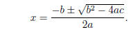
Note that there will be either one, two, or potentially no roots, depending on the value of the_______________ ,
b² − 4ac.

Examples. Find the roots of each of the following polynomials.

1. y² + 4y − 21 = 0

2. 2r² − 5r + 1 = 2r − 1

3. x² + x + 3 = 0 (Note: what’s going on here?!!?)
 

In this last case we see that since the solution requires taking the square root of a negative number, we
have NO real roots! (The roots lie in the collection of ____________ numbers, which are defined via
the value i =sqrt(−1).
 

We can see solutions to quadratic equations graphically, as well.

Examples. On separate axes, graph the expressions in (1) and (3) from the previous example.

Is it any coincidence the zeroes of the graphs appeared where they did?

The following fact will be useful to keep in mind when we begin talking about higher degree polynomial
equations. We say that the polynomial q is a __________ of the polynomial p if when we long-divide p
by q the remainder is 0.

The Factor Theorem. The linear term x − r is a factor of the polynomial p(x) if and only if r is a
root of the polynomial (that is, if p(r) = 0).

Proof. We will make clever use of long division! Let’s complete this proof together in the space below...



You should now be ready to tackle Homework 3.1.1 on-line; this homework is due by Friday, October
17th.